A python library for time-series smoothing and outlier detection in a vectorized way.

• 去噪
• 异常值剔除
• 保留原始数据中存在的时间模式

tsmoothie 平滑

平滑技术

tsmoothie 使用的平滑技术：

• Exponential Smoothing(指数平滑)
• Convolutional Smoothing(卷积平滑)
  • constant: window types
  • hanning: window types
  • hamming: window types
  • bartlett: window types
  • blackman: window types
• Spectral Smoothing with Fourier Transform(傅里叶变换的频谱平滑)
• Polynomial Smoothing(多项式平滑)
• Spline Smoothing(样条平滑)
  • linear
  • cubic
  • natural
  • cubic
• Gaussian Smoothing(高斯平滑)
• Binner Smoothing(分箱平滑)
• LOWESS(局部加权回归散点平滑法)
• Seasonal Decompose Smoothing(季节性分解)
  • convolution
  • lowess
  • natural
  • cubic
  • spline
• Kalman Smoothing(卡尔曼平滑) with customizable components
  • level
  • trend
  • seasonality
  • long seasonality

指数平滑

LOWESS

二维变量之间的关系研究是很多统计方法的基础，例如回归分析通常会从一元回归讲起，然后再扩展到多元情况。 局部加权回归散点平滑法（locally weighted scatterplot smoothing，LOWESS 或 LOESS）是查看二维变量之间关系的一种有力工具。

LOWESS 主要思想是取一定比例的局部数据，在这部分子集中拟合多项式回归曲线， 这样便可以观察到数据在局部展现出来的规律和趋势； 而通常的回归分析往往是根据全体数据建模，这样可以描述整体趋势， 但现实生活中规律不总是（或者很少是）教科书上告诉的一条直线。 将局部范围从左往右依次推进，最终一条连续的曲线就被计算出来了。 显然，曲线的平滑程度与选取数据比例有关：比例越少， 拟合越不平滑（因为过于看重局部性质），反之越平滑

区间计算

tsmoothie 提供了作为平滑过程结果的区间计算，这对于识别时间序列中的异常值非常有用。 区间类型有：

• sigma interval
• confidence interval
• predictions interval
• kalman interval

tsmoothie 可以进行滑动平滑的方法来模拟在线使用。 这可以将时间序列分成大小相等的部分并独立平滑它们。 与往常一样，此功能通过 WindowWrapper 类以矢量化方式实现

Bootstrap 算法

tsmoothie 可以通过 BootstrappingWrapper 类操作时序引导，用到的 Bootstrap 算法有：

• none overlapping block bootstrap
• moving block bootstrap
• circular block bootstrap
• stationary bootstrap

tsmoothie 安装

$ pip install tsmoothie

tsmoothie 使用

tsmoothie 平滑 demo

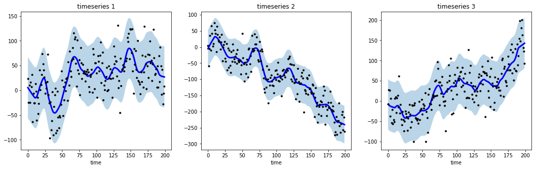
随机游走数据平滑

import numpy as np
import matplotlib.pyplot as plt
from tsmoothie.utils_func import sim_randomwalk
from tsmoothie.smoother import LowessSmoother

# ------------------------------
# generate 3 randomwalks of length 200 
# ------------------------------
np.random.seed(123)
data = sim_randomwalk(
    n_series = 3,
    timesteps = 200,
    process_noise = 10,
    measure_noise = 30,
)

# ------------------------------
# Smoothing
# ------------------------------
# operate smoothing
smoother = LowessSmoother(smooth_fraction = 0.1, iterations = 1)
smoother.smooth(data)
# generate intervals
low, up = smoother.get_intervals("prediction_interval")

# ------------------------------
# plot the smoothed timeseries with intervals 
# ------------------------------
plt.figure(figsize = (18, 5))
for i in range(3):
    plt.subplot(1, 3, i + 1)
    plt.plot(smoother.smooth_data[i], linewidth = 3, color = "blue")
    plt.plot(smoother.data[i], ".k")
    plt.title(f"timeseries {i + 1}")
    plt.xlabel("time")
    plt.fill_between(
        range(len(smoother.data[i])),
        low[i],
        up[i],
        alpha = 0.3,
    )

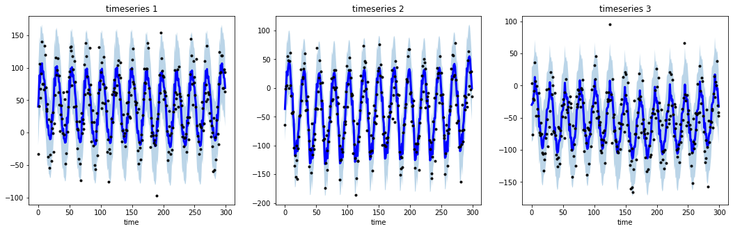
季节性数据平滑

# import libraries
import numpy as np
import matplotlib.pyplot as plt
from tsmoothie.utils_func import sim_seasonal_data
from tsmoothie.smoother import DecomposeSmoother

# ------------------------------
# generate 3 periodic timeseries of lenght 300
# ------------------------------
np.random.seed(123)
data = sim_seasonal_data(
    n_series = 3, 
    timesteps = 300, 
    freq = 24, 
    measure_noise = 30
)

# ------------------------------
# Smoothing
# ------------------------------
# operate smoothing
smoother = DecomposeSmoother(
    smooth_type = 'lowess', 
    periods = 24,
    smooth_fraction = 0.3
)
smoother.smooth(data)
# generate intervals
low, up = smoother.get_intervals('sigma_interval')

# ------------------------------
# plot the smoothed timeseries with intervals 
# ------------------------------
plt.figure(figsize = (18, 5))
for i in range(3):
    plt.subplot(1, 3, i + 1)
    plt.plot(smoother.smooth_data[i], linewidth = 3, color = 'blue')
    plt.plot(smoother.data[i], '.k')
    plt.title(f"timeseries {i+1}")
    plt.xlabel('time')
    plt.fill_between(
        range(len(smoother.data[i])), 
        low[i], 
        up[i], 
        alpha = 0.3
    )

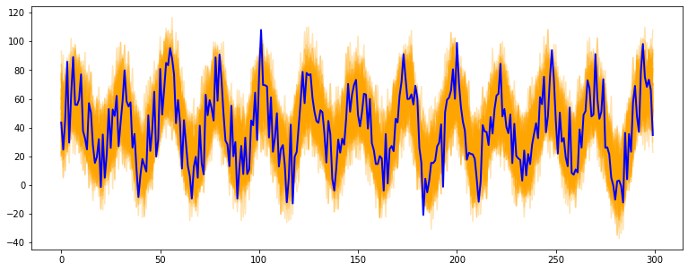
tsmoothie Bootstrap demo

# import libraries
import numpy as np
import matplotlib.pyplot as plt
from tsmoothie.utils_func import sim_seasonal_data
from tsmoothie.smoother import ConvolutionSmoother
from tsmoothie.bootstrap import BootstrappingWrapper

# ------------------------------
# generate a periodic timeseries of lenght 300 
# ------------------------------
np.random.seed(123)
data = sim_seasonal_data(
    n_series = 1, 
    timesteps = 300, 
    freq = 24, 
    measure_noise = 15
)

# ------------------------------
# operate bootstrap 
# ------------------------------
bts = BootstrappingWrapper(
    ConvolutionSmoother(
        window_len = 8, 
        window_type = 'ones'
    ), 
    bootstrap_type = 'mbb', 
    block_length = 24
)
bts_samples = bts.sample(data, n_samples = 100)

# ------------------------------
# plot the bootstrapped timeseries
# ------------------------------
plt.figure(figsize = (13, 5))
plt.plot(bts_samples.T, alpha = 0.3, c = 'orange')
plt.plot(data[0], c = 'blue', linewidth = 2)

时间序列平滑以更好地聚类

时间序列平滑以更好地预测

降低传感器中的噪声以更好地预测太阳能电池板的发电量

时间序列数据

• 房子每天的煤气消耗量，$m^{3}$
• 房子每天的用电量，$kWh$
  • 负值表示太阳能超出了房子的用电量
• 直流转交流转换器上功率计的日值。这是当前累积的太阳能发电量。 不需要累积值，而是需要绝对的每日值，因此，进行简单的微分操作。 这是预测的目标

时间序列数据平滑

Kalman Filter

时间序列异常检测

极端事件的时间序列预处理

深度学习中的时间序列 Bootstrap

参考

• GitHub tsmoothie
• 用局部加权回归散点平滑法观察二维变量之间的关系
• Time Series Smoothing for better Forecasting