Statsmodels
wangzf / 2022-05-02
statistical models, hypothesis tests, and data exploration
安装
依赖
- Python >= 3.7
- NumPy >= 1.17
- SciPy >= 1.3
- Pandas >= 1.0
- Patsy >= 0.5.2
- Cython
conda
$ conda install -c conda-forge statsmodels
PyPI
$ pip install statsmodels
使用
简单线性回归
statsmodels 支持模型使用以下两种风格:
- R 语言公式风格
- pandas.DataFrame/numpy array
公式风格
import numpy as np
import statsmodels.api as sm
import statsmodels.formula.api as smf

# data
data = sm.datasets.get_rdataset("Guerry", "HistData").data
print(data)

# regression model
results = smf.ols(
    "Lottery ~ Literacy + np.log(Pop1831)",
    data = data
).fit()
print(results.summary())
print(dir(results))
print(results.__doc__)
    dept Region    Department  Crime_pers  ...  Prostitutes  Distance  Area  Pop1831
0      1      E           Ain       28870  ...           13   218.372  5762   346.03
1      2      N         Aisne       26226  ...          327    65.945  7369   513.00
2      3      C        Allier       26747  ...           34   161.927  7340   298.26
3      4      E  Basses-Alpes       12935  ...            2   351.399  6925   155.90
4      5      E  Hautes-Alpes       17488  ...            1   320.280  5549   129.10
..   ...    ...           ...         ...  ...          ...       ...   ...      ...
81    86      W        Vienne       15010  ...           18   170.523  6990   282.73
82    87      C  Haute-Vienne       16256  ...            7   198.874  5520   285.13
83    88      E        Vosges       18835  ...           43   174.477  5874   397.99
84    89      C         Yonne       18006  ...          272    81.797  7427   352.49
85   200    NaN         Corse        2199  ...            1   539.213  8680   195.41

[86 rows x 23 columns]
                            OLS Regression Results
==============================================================================
Dep. Variable:                Lottery   R-squared:                       0.348
Model:                            OLS   Adj. R-squared:                  0.333
Method:                 Least Squares   F-statistic:                     22.20
Date:                Thu, 17 Nov 2022   Prob (F-statistic):           1.90e-08
Time:                        00:01:21   Log-Likelihood:                -379.82
No. Observations:                  86   AIC:                             765.6
Df Residuals:                      83   BIC:                             773.0
Df Model:                           2
Covariance Type:            nonrobust
===================================================================================
                      coef    std err          t      P>|t|      [0.025      0.975]
-----------------------------------------------------------------------------------
Intercept         246.4341     35.233      6.995      0.000     176.358     316.510
Literacy           -0.4889      0.128     -3.832      0.000      -0.743      -0.235
np.log(Pop1831)   -31.3114      5.977     -5.239      0.000     -43.199     -19.424
==============================================================================
Omnibus:                        3.713   Durbin-Watson:                   2.019
Prob(Omnibus):                  0.156   Jarque-Bera (JB):                3.394
Skew:                          -0.487   Prob(JB):                        0.183
Kurtosis:                       3.003   Cond. No.                         702.
==============================================================================

Notes:
[1] Standard Errors assume that the covariance matrix of the errors is correctly specified.
['HC0_se', 'HC1_se', 'HC2_se', 'HC3_se', '_HCCM', '__class__', '__delattr__', '__dict__', '__dir__', '__doc__', '__eq__', '__format__', '__ge__', '__getattribute__', '__gt__', '__hash__', '__init__', '__init_subclass__', '__le__', '__lt__', '__module__', '__ne__', '__new__', '__reduce__', '__reduce_ex__', '__repr__', '__setattr__', '__sizeof__', '__str__', '__subclasshook__', '__weakref__', '_abat_diagonal', '_cache', '_data_attr', '_data_in_cache', '_get_robustcov_results', '_is_nested', '_use_t', '_wexog_singular_values', 'aic', 'bic', 'bse', 'centered_tss', 'compare_f_test', 'compare_lm_test', 'compare_lr_test', 'condition_number', 'conf_int', 'conf_int_el', 'cov_HC0', 'cov_HC1', 'cov_HC2', 'cov_HC3', 'cov_kwds', 'cov_params', 'cov_type', 'df_model', 'df_resid', 'diagn', 'eigenvals', 'el_test', 'ess', 'f_pvalue', 'f_test', 'fittedvalues', 'fvalue', 'get_influence', 'get_prediction', 'get_robustcov_results', 'info_criteria', 'initialize', 'k_constant', 'llf', 'load', 'model', 'mse_model', 'mse_resid', 'mse_total', 'nobs', 'normalized_cov_params', 'outlier_test', 'params', 'predict', 'pvalues', 'remove_data', 'resid', 'resid_pearson', 'rsquared', 'rsquared_adj', 'save', 'scale', 'ssr', 'summary', 'summary2', 't_test', 't_test_pairwise', 'tvalues', 'uncentered_tss', 'use_t', 'wald_test', 'wald_test_terms', 'wresid']
Results class for for an OLS model.

Parameters
----------
model : RegressionModel
    The regression model instance.
params : ndarray
    The estimated parameters.
normalized_cov_params : ndarray
    The normalized covariance parameters.
scale : float
    The estimated scale of the residuals.
cov_type : str
    The covariance estimator used in the results.
cov_kwds : dict
    Additional keywords used in the covariance specification.
use_t : bool
    Flag indicating to use the Student's t in inference.
**kwargs
    Additional keyword arguments used to initialize the results.

See Also
--------
RegressionResults
    Results store for WLS and GLW models.

Notes
-----
Most of the methods and attributes are inherited from RegressionResults.
The special methods that are only available for OLS are:

- get_influence
- outlier_test
- el_test
- conf_int_el
numpy array 风格
import numpy as np
import statsmodels.api as sm

# data
nobs = 100
X = np.random.random((nobs, 2))
X = sm.add_constant(X)
beta = [1, 0.1, 0.5]
e = np.random.random(nobs)
y = np.dot(X, beta) + e

# regression model
results = sm.OLS(y, X).fit()
print(results.summary())
                           OLS Regression Results
==============================================================================
Dep. Variable:                      y   R-squared:                       0.178
Model:                            OLS   Adj. R-squared:                  0.161
Method:                 Least Squares   F-statistic:                     10.51
Date:                Wed, 02 Nov 2022   Prob (F-statistic):           7.41e-05
Time:                        17:12:45   Log-Likelihood:                -20.926
No. Observations:                 100   AIC:                             47.85
Df Residuals:                      97   BIC:                             55.67
Df Model:                           2
Covariance Type:            nonrobust
==============================================================================
                 coef    std err          t      P>|t|      [0.025      0.975]
------------------------------------------------------------------------------
const          1.4713      0.075     19.579      0.000       1.322       1.620
x1             0.1045      0.105      1.000      0.320      -0.103       0.312
x2             0.4831      0.107      4.503      0.000       0.270       0.696
==============================================================================
Omnibus:                       39.684   Durbin-Watson:                   1.848
Prob(Omnibus):                  0.000   Jarque-Bera (JB):                6.503
Skew:                           0.096   Prob(JB):                       0.0387
Kurtosis:                       1.766   Cond. No.                         5.09
==============================================================================

Notes:
[1] Standard Errors assume that the covariance matrix of the errors is correctly specified.
详细使用
载入模块和函数
import pandas as pd
import statsmodels.api as sm
from patsy import dmatrices
数据
df = sm.datasets.get_rdataset("Guerry", "HistData").data
vars = ["Department", "Lottery", "Literacy", "Wealth", "Region"]
df = df[vars]
df = df.dropna()
df[-5:]
      Department  Lottery  Literacy  Wealth Region
80        Vendee       68        28      56      W
81        Vienne       40        25      68      W
82  Haute-Vienne       55        13      67      C
83        Vosges       14        62      82      E
84         Yonne       51        47      30      C
构造设计矩阵
y, X = dmatrices(
    "Lottery ~ Literacy + Wealth + Region",
    data = df,
    return_type = "dataframe"
)
y[:3]
x[:3]
   Lottery
0     41.0
1     38.0
2     66.0

   Intercept  Region[T.E]  Region[T.N]  ...  Region[T.W]  Literacy  Wealth
0        1.0          1.0          0.0  ...          0.0      37.0    73.0
1        1.0          0.0          1.0  ...          0.0      51.0    22.0
2        1.0          0.0          0.0  ...          0.0      13.0    61.0

[3 rows x 7 columns]
模型
model = sm.OLS(y, X)
result = model.fit()
print(result.summary())
                            OLS Regression Results
==============================================================================
Dep. Variable:                Lottery   R-squared:                       0.338
Model:                            OLS   Adj. R-squared:                  0.287
Method:                 Least Squares   F-statistic:                     6.636
Date:                Wed, 02 Nov 2022   Prob (F-statistic):           1.07e-05
Time:                        17:12:43   Log-Likelihood:                -375.30
No. Observations:                  85   AIC:                             764.6
Df Residuals:                      78   BIC:                             781.7
Df Model:                           6
Covariance Type:            nonrobust
===============================================================================
                  coef    std err          t      P>|t|      [0.025      0.975]
-------------------------------------------------------------------------------
Intercept      38.6517      9.456      4.087      0.000      19.826      57.478
Region[T.E]   -15.4278      9.727     -1.586      0.117     -34.793       3.938
Region[T.N]   -10.0170      9.260     -1.082      0.283     -28.453       8.419
Region[T.S]    -4.5483      7.279     -0.625      0.534     -19.039       9.943
Region[T.W]   -10.0913      7.196     -1.402      0.165     -24.418       4.235
Literacy       -0.1858      0.210     -0.886      0.378      -0.603       0.232
Wealth          0.4515      0.103      4.390      0.000       0.247       0.656
==============================================================================
Omnibus:                        3.049   Durbin-Watson:                   1.785
Prob(Omnibus):                  0.218   Jarque-Bera (JB):                2.694
Skew:                          -0.340   Prob(JB):                        0.260
Kurtosis:                       2.454   Cond. No.                         371.
==============================================================================

Notes:
[1] Standard Errors assume that the covariance matrix of the errors is correctly specified.
result.params
result.rsquared
Intercept      38.651655
Region[T.E]   -15.427785
Region[T.N]   -10.016961
Region[T.S]    -4.548257
Region[T.W]   -10.091276
Literacy       -0.185819
Wealth          0.451475
dtype: float64

0.337950869192882
模型诊断和测试
sm.stats.linear_rainbow(result)
print(sm.stats.linear_rainbow.__doc__)
# (F-statistic, p-value)
(0.8472339976156916, 0.6997965543621643)
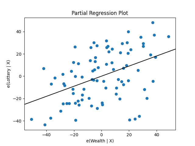
sm.graphics.plot_partregress(
    "Lottery",
    "Wealth",
    ["Region", "Literacy"],
    data = df,
    obs_labels = False
)
回归与线性模型
时间序列分析
ARMA
statsmodels.tsa
- Univariate
- autoregressive models(AR)
- vector autoregressive models(VAR)
- autoregressive moving average models(ARMA)
- Non-linear models
- Markov switching dynamic regression and autoregression
- 描述性统计量
- autocorrelation: 自相关图
- partal autocorrelation: 偏自相关图
- periodogram: 周期图
- ARMA 相关的理论属性或过程
- 使用 AR 和 MA 滞后多项式(lag-polynomials)的方法
- 相关的统计检验
- 一些有用的函数
statsmodels.tsa 命名空间中的模块结构:
- stattools
- ar_model
- arima.model
- statspace
- vector_ar
- arma_process
- sandbox.tsa.fftarma
- tsatools
- filters
- regime_switching
估计
- 极大似然估计、条件极大似然估计(exact or condition Maximum Likelihood)
- 条件最小二乘(conditional least-quares)
- 卡尔曼滤波(Kalman Filter)或直接滤波器(direct filters.)
指数平滑 Exponential Smoothing
Holt Winter’s Exponential Smoothing
Simple Exponential Smoothing
Holt’s Exponential Smoothing
自相关系数和偏自相关系数计算
import statsmodels.api as sm

X = [2, 3, 4, 3, 8, 7]
print(sm.tsa.stattools.acf(X, nlags = 1, adjusted = True))
[1, 0.3559322]
自相关图和偏自相关图绘制
import numpy as np
import pandas as pd
import akshare as ak
from matplotlib import pyplot as plt
from statsmodels.graphics.tsaplots import plot_acf, plot_pacf

np.random.seed(123)

# -------------- 准备数据 --------------
# 白噪声
white_noise = np.random.standard_normal(size=1000)

# 随机游走
x = np.random.standard_normal(size=1000)
random_walk = np.cumsum(x)

# GDP
df = ak.macro_china_gdp()
df = df.set_index('季度')
df.index = pd.to_datetime(df.index)
gdp = df['国内生产总值-绝对值'][::-1].astype('float')

# GDP DIFF
gdp_diff = gdp.diff(4).dropna()

# -------------- 绘制图形 --------------
fig, ax = plt.subplots(4, 2)
fig.subplots_adjust(hspace = 0.5)

plot_acf(white_noise, ax = ax[0][0])
ax[0][0].set_title('ACF(white_noise)')
plot_pacf(white_noise, ax = ax[0][1])
ax[0][1].set_title('PACF(white_noise)')

plot_acf(random_walk, ax = ax[1][0])
ax[1][0].set_title('ACF(random_walk)')
plot_pacf(random_walk, ax = ax[1][1])
ax[1][1].set_title('PACF(random_walk)')

plot_acf(gdp, ax = ax[2][0])
ax[2][0].set_title('ACF(gdp)')
plot_pacf(gdp, ax = ax[2][1])
ax[2][1].set_title('PACF(gdp)')

plot_acf(gdp_diff, ax = ax[3][0])
ax[3][0].set_title('ACF(gdp_diff)')
plot_pacf(gdp_diff, ax = ax[3][1])
ax[3][1].set_title('PACF(gdp_diff)')

plt.show()