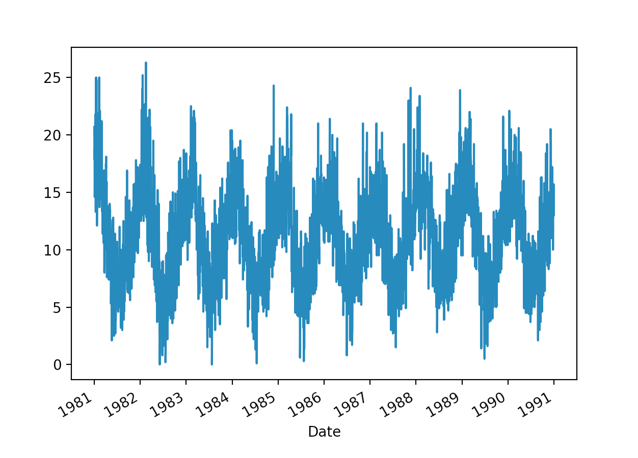
时间序列示例数据
import pandas as pd
import matplotlib.pyplot as plt

series = pd.read_csv(
    "https://raw.githubusercontent.com/jbrownlee/Datasets/master/daily-min-temperatures.csv",
    header = 0,
    index_col = 0,
    parse_dates = True,
    date_parser = lambda dates: pd.to_datetime(dates, format = '%Y-%m-%d'),
    squeeze = True
)
print(series.head())
Date
1981-01-01    20.7
1981-01-02    17.9
1981-01-03    18.8
1981-01-04    14.6
1981-01-05    15.8
Name: Temp, dtype: float64
series.plot()
plt.show()
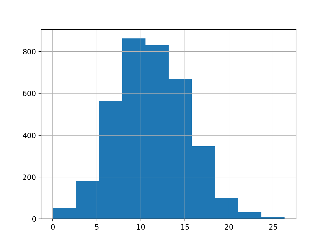
series.hist()
plt.show()
标准化和中心化
标准化
标准化是使时间序列中的数值符合平均值为 0,标准差为 1。具体来说,
对于给定的时间序列 $\{x_{1}, x_{2}, \ldots, x_{t}, \ldots, x_{T}\}$,
有如下公式:
$$\hat{x}_{t} = \frac{x_{t} - mean(\{x_{t}\}_{t}^{T})}{std(\{x_{t}\}_{t}^{T})}$$
from pandas import read_csv
from sklearn.preprocessing import StandarScaler
from math import sqrt

# Data
series = pd.read_csv(
    "daily-minimum-temperatures-in-me.csv",
    header = 0,
    index_col = 0
)
print(series.head())
values = series.values
values = values.reshape((len(values), 1))

# Standardization
scaler = StandardScaler()
scaler = scaler.fit(values)
print("Mean: %f, StandardDeviation: %f" % (scaler.mean_, sqrt(scaler.var_)))

# 标准化
normalized = scaler.transform(values)
for i in range(5):
    print(normalized[i])

# 逆变换
inversed = scaler.inverse_transform(normalized)
for i in range(5):
    print(inversed[i])
normalized.plot()

inversed.plot()

中心化
标准化的目标是将原始数据分布转换为标准正态分布,它和整体样本分布有关, 每个样本点都能对标准化产生影响。这里,如果只考虑将均值缩放到 0, 不考虑标准差的话,为数据中心化处理:
$$\hat{x}_{t} = x_{t} - mean(\{x_{t}\}_{t}^{T})$$
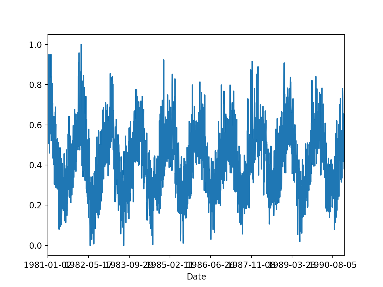
归一化
归一化是将样本的特征值转换到同一范围(量纲)下,把数据映射到 $[0, 1]$ 或 $[-1, 1]$ 区间内,
它仅由变量的极值所决定,其主要是为了数据处理方便而提出来的。
归一化
把数据映射到 $[0, 1]$ 范围之内进行处理,可以更加便捷快速。具体公式如下:
$$\hat{x}_{t} = \frac{x_{t} - min(\{x_{t}\}_{t}^{T})}{max(\{x_{t}\}_{t}^{T}) - min(\{x_{t}\}_{t}^{T})}$$
import pandas as pd
from sklearn.preprocessing import MinMaxScaler
# Data
series = pd.read_csv(
"daily-minimum-temperautures-in-me.csv",
header = 0,
index_col = 0
)
print(series.head())
values = series.values
values = values.reshape((len(values), 1))
# Normalization
scaler = MinMaxScaler(feature_range = (0, 1))
scaler = scaler.fit(values)
print("Min: %f, Max: %f" % (scaler.data_min_, scaler.data_max_))
# 正规化
normalized = scaler.transform(values)
for i in range(5):
print(normalized[i])
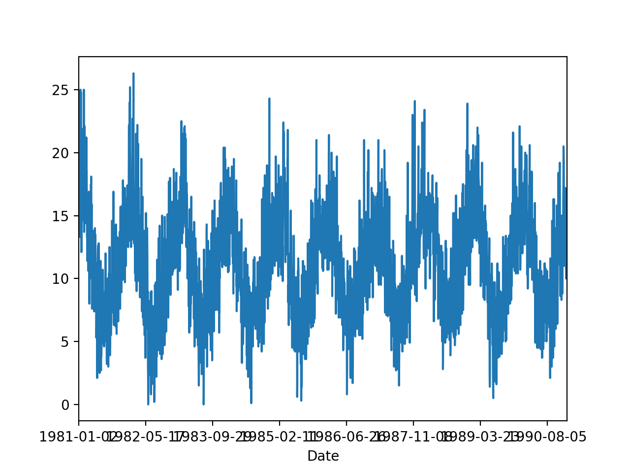
# 逆变换
inversed = scaler.inverse_transform(normalized)
for i in range(5):
print(inversed[i])
normalized.plot()
inversed.plot()
平均归一化
$$\hat{x}_{t} = \frac{x_{t} - mean(\{x_{t}\}_{t}^{T})}{max(\{x_{t}\}_{t}^{T}) - min(\{x_{t}\}_{t}^{T})}$$
什么时候用归一化?什么时候用标准化?
- 如果对输出结果范围有要求,用归一化;
- 如果数据较为稳定,不存在极端的最大最小值,用归一化;
- 如果数据存在异常值和较多噪音,用标准化,可以间接通过中心化避免异常值和极端值的影响。
时间序列聚合
通常来自不同数据源的时间轴常常无法一一对应, 此时就要用到改变时间频率的方法进行数据处理. 由于无法改变实际测量数据的频率, 我们能做的是改变数据收集的频率。
重采样(resampling)指的是将时间序列从一个频率转换到另一个频率的处理过程。 是对原样本重新处理的一个方法,是一个对常规时间序列数据重采样和频率转换的便捷的方法。 将高频率的数据聚合到低频率称为降采样(down sampling), 而将低频率数据转换到高频率则称为升采样(up sampling)。
- 升采样(up sampling): 在某种程度上是凭空获得更高频率数据的方式, 不增加额外的信息;
- 降采样(down sampling): 减少数据收集的频率, 也就是从原始数据中抽取子集的方式。
Pandas 重采样
API
pd.DataFrame.resample(
    rule,
    how = None,
    axis = 0,
    fill_method = None,
    closed = None,
    label = None,
    convention = 'start',
    kind = None,
    loffset = None,
    limit = None,
    base = 0,
    on = None,
    level = None
)

pd.Series.resample(
    rule,
    how = None,
    axis = 0,
    fill_method = None,
    closed = None,
    label = None,
    convention = 'start',
    kind = None,
    loffset = None,
    limit = None,
    base = 0,
    on = None,
    level = None
)
主要参数说明:
rule:DateOffset,Timedeltaorstr- 表示重采样频率,例如
"M"、"5min","Second(15)"
how:- 用于产生聚合值的函数名或数组函数
- 例如
'mean'、'ohlc'、'np.max'等,默认是'mean'。 其他常用的值有:'first'、'last'、'median'、'max'、'min'
axis:0or'index'1or'columns'- default
0
fill_method:- str, default None
- 升采样时如何插值,比如
ffill、bfill等
closed:- 在降采样时,各时间段的哪一段是闭合的
'right'或'left',默认'right'
label:- {
'right','left'}, defaultNone - 在降采样时,如何设置聚合值的标签,例如,9:30-9:35 会被标记成 9:30 还是 9:35, 默认9:35
- {
convention:- 当重采样时期时,将低频率转换到高频率所采用的约定
- {
'start','end','s','e'}, default'start'
kind:- 聚合到时期(‘period’)或时间戳(’timestamp’),默认聚合到时间序列的索引类型
'timestamp','period', defaultNone
loffset:- 面元标签的时间校正值,比如’-1s’或Second(-1)用于将聚合标签调早1秒
- timedelta, default None
limit:- 在向前或向后填充时,允许填充的最大时期数
- int, default None
升采样
API:
.resample().ffill().resample().bfill().resample().pad().resample().nearest().resample().fillna().resample().asfreq().resample().interpolate()
降采样
API:
.resample().<func>().resample.count().resample.nunique().resample.first().resample.last().resample.ohlc().resample.prod().resample.size().resample.sem().resample.std().resample.var().resample.quantile().resample.mean().resample.median().resample.min().resample.max().resample.sum()
Function application
API:
.resample().apply(custom_resampler): 自定义函数.resample().aggregate().resample().transfrom().resample().pipe()
Indexing 和 iteration
API:
.__iter__.groups.indicesget_group()
稀疏采样
API:
SciPy 重采样
API
import scipy

scipy.signal.resample(
    x,
    num,
    t = None,
    axis = 0,
    window = None,
    domain = 'time'
)
参数解释:
x: 待重采样的数据num: 重采样的点数,int型t: 如果给定t,则假定它是与x中的信号数据相关联的等距采样位置axis: 对哪个轴重采样,默认是 0
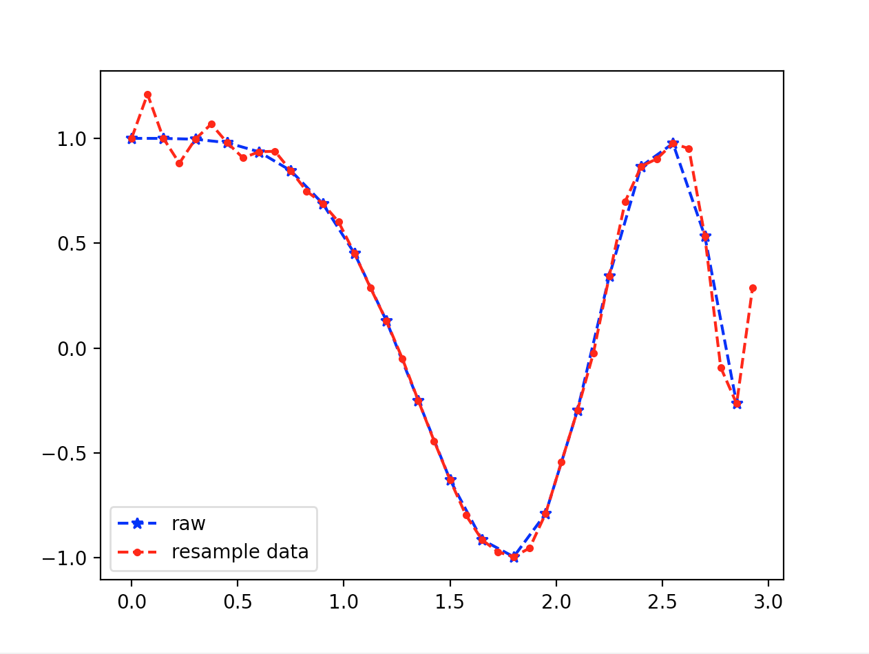
升采样
import numpy as np
import matplotlib.pyplot as plt
from scipy import signal

# 原始数据
t = np.linspace(0, 3, 20, endpoint = False)
y  = np.cos(t ** 2)

# 升采样, 20 个点采 40 个点
re_y = singal.resample(y, 40)
t_new = np.linspace(0, 3, len(re_y), endpoint = False)

# plot
plt.plot(t, y, "b*--", label = "raw")
plt.plot(t_new, re_y, "r.--", lable = "resample data")
plt.legend()
plt.show()
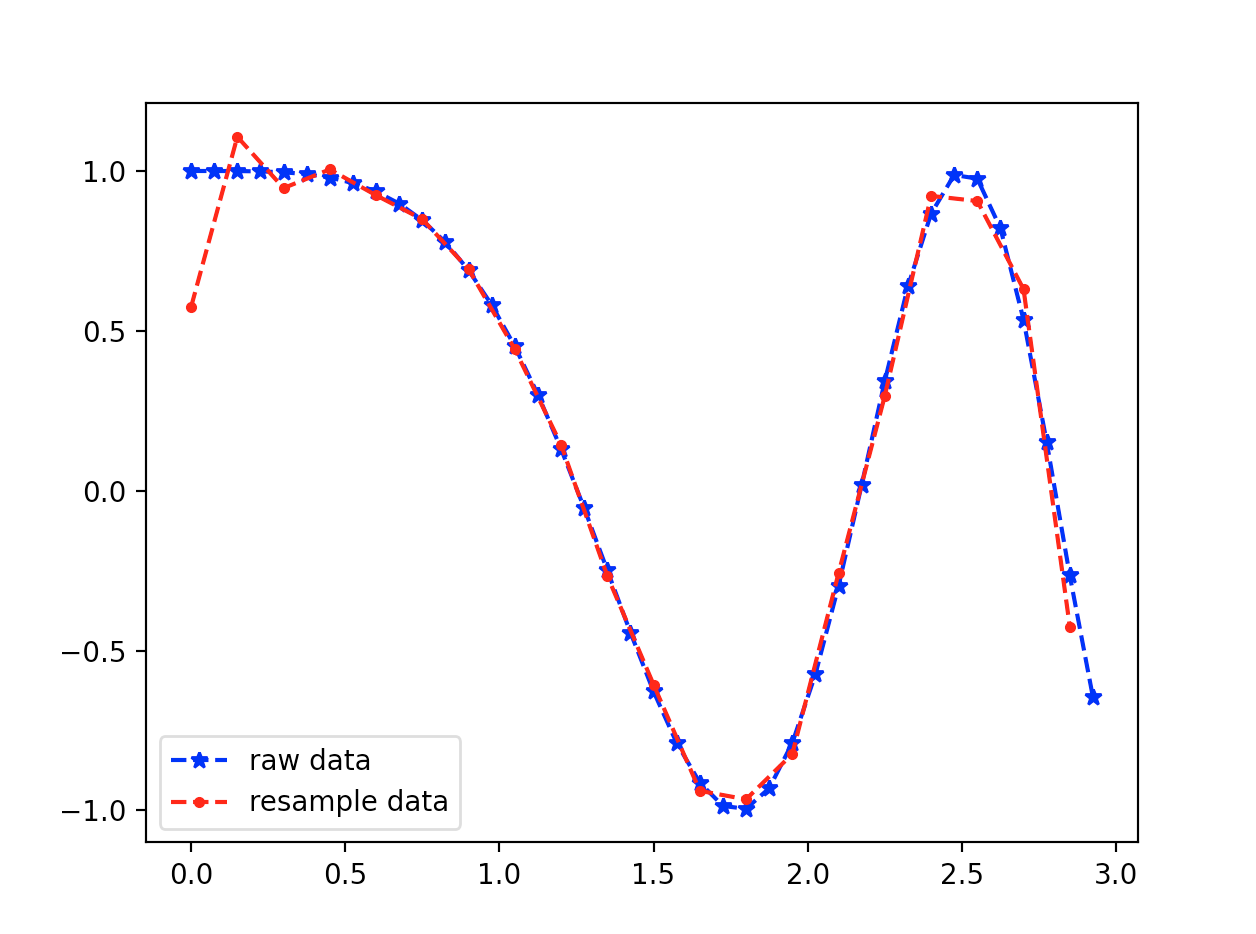
降采样
import numpy as np
import matplotlib.pyplot as plt
from scipy import signal

# 原始数据
t = np.linspace(0, 3, 40, endpoint = False)
y = np.cos(t ** 2)

# 降采样, 40 个点采 20 个点
re_y = signal_resample(y, 20)
t_new = np.linspace(0, 3, len(re_y), endpoint = False)

# plot
plt.plot(t, y, "b*--", label = "raw data")
plt.plot(t_new, re_y, "r.--", label = "resample data")
plt.legend()
plt.show()
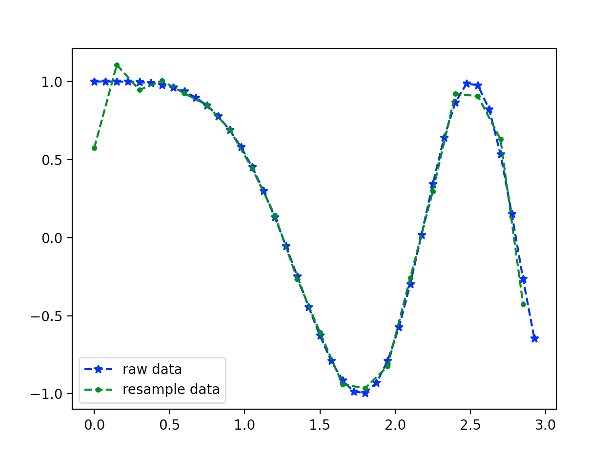
等间隔采样
import numpy as np
import matplotlib.pyplot as plt
from scipy import signal

# 原始数据
t = np.linspace(0, 3, 40, endpoint = False)
y = np.cos(t ** 2)

# 等间隔降采样,40 个点采 20 个点
re_y, re_t = signal.resample(y, 20, t = t)

# plot
plt.plot(t, y, "b*--", label = "raw data")
plt.plot(re_t, re_y, "g.--", label = "resample data")
plt.legend()
plt.show()
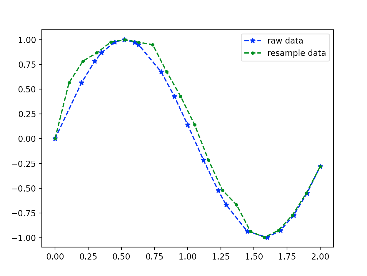
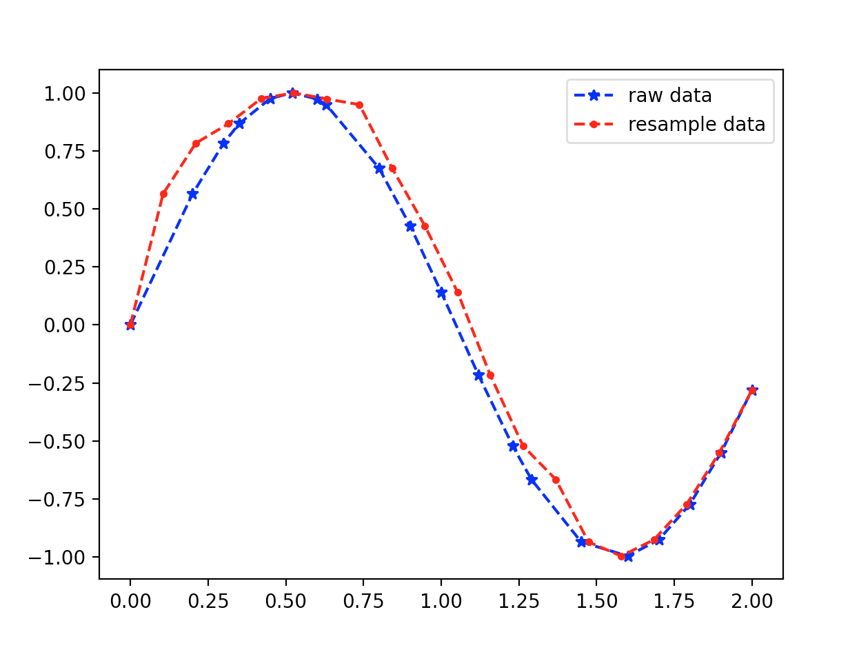
不等间隔采样
原始数据不等间隔,采样成等间隔的点(点数不变)
import numpy as np
import matplotlib.pyplot as plt
from scipy import signal

# 原始数据
t = np.array([
    0, 2, 3, 3.5, 4.5,
    5.2, 6, 6.3, 8, 9,
    10, 11.2, 12.3, 12.9, 14.5,
    16, 17, 18, 19, 20]) / 10
x = np.sin(3 * t)

# 重采样为等间隔
t1 = np.linspace(0, 2, 20, endpoint = True)
re_x, re_t = signal.resample(x, 20, t = t1)

# plot
plt.plot(t, x, 'b*--', label = 'raw data')
plt.plot(re_t, re_x, 'g.--', label = 'resample data')
plt.legend()
plt.show()
import numpy as np
import matplotlib.pyplot
from scipy import signal

# 原始数据
t = np.array([
    0, 2, 3, 3.5, 4.5,
    5.2, 6, 6.3, 8, 9,
    10, 11.2, 12.3, 12.9, 14.5,
    16, 17, 18, 19, 20])/10
x = np.sin(3 * t)

# 重采样
t1 = np.linspace(0, 2, 20, endpoint = True)
re_x = signal.resample(x, 20)

plt.plot(t, x, 'b*--', label = 'raw data')
plt.plot(t1, re_x, 'r.--', label = 'resample data')
plt.legend()
plt.show()
时间序列缺失处理
最常用的处理缺失值的方法包括填补(imputation) 和删除(deletion)两种
常见的数据填补(imputation)方法:
- forward fill 和 backward fill
- 根据缺失值前/后的最近时间点数据填补当前缺失值
- Moving Average
- Interpolation
- 插值方法要求数据和邻近点之间满足某种拟合关系, 因此插值法是一种先验方法且需要代入一些业务经验
forward 和 backward fill
Moving Average
Pandas 插值算法
Pandas 中缺失值的处理
- Python 缺失值类型
Nonenumpy.nanNaNNaT
- 缺失值配置选项
- 将
inf和-inf当作NApandas.options.mod.use_inf_as_na = True
- 将
- 缺失值检测
pd.isna().isna()pd.notna().notna()
- 缺失值填充
.fillna().where(pd.notna(df), dict(), axis = "columns").ffill().fillna(method = "ffill", limit = None)
.bfill().fillna(method = "bfill", limit = None)
.interpolate(method).replace(, method)
- 缺失值删除
.dropna(axis)
缺失值插值算法 API
pandas.DataFrame.interpolate
pandas.DataFrame.interpolate(
   method = 'linear',
   axis = 0,
   limit = None,
   inplace = False,
   limit_direction = 'forward',
   limit_area = None,
   downcast = None,
   **kwargs
)
methodlinear: 等间距插值, 支持多多索引time: 对索引为不同分辨率时间序列数据插值index,value: 使用索引的实际数值插值pad: 使用其他不为NaN的值插值nearest: 参考scipy.iterpolate.interp1d中的插值算法zero: 参考scipy.iterpolate.interp1d中的插值算法slinear: 参考scipy.iterpolate.interp1d中的插值算法quadratic: 参考scipy.iterpolate.interp1d中的插值算法cubic: 参考scipy.iterpolate.interp1d中的插值算法spline: 参考scipy.iterpolate.interp1d中的插值算法barycentric: 参考scipy.iterpolate.interp1d中的插值算法polynomial: 参考scipy.iterpolate.interp1d中的插值算法krogh:scipy.interpolate.KroghInterpolator
piecewise_polynomialsplinescipy.interpolate.CubicSpline
pchipscipy.interpolate.PchipInterpolator
akimascipy.interpolate.Akima1DInterpolator
from_derivativesscipy.interpolate.BPoly.from_derivatives
axis:- 1
- 0
limit: 要填充的最大连续NaN数量, :math:>0inplace: 是否在原处更新数据limit_direction: 缺失值填充的方向- forward
- backward
- both
limit_area: 缺失值填充的限制区域- None
- inside
- outside
downcast: 强制向下转换数据类型- infer
- None
**kwargs- 传递给插值函数的参数
s = pd.Series([])
df = pd.DataFrame({})

s.interpolate(args)
df.interpolate(args)
df[""].interpolate(args)
Scipy 插值算法
- scipy.interpolate.Akima1DInterpolator
- 三次多项式插值
- scipy.interpolate.BPoly.from_derivatives
- 多项式插值
- scipy.interpolate.interp1d
- 1-D 函数插值
- scipy.interpolate.KroghInterpolator
- 多项式插值
- scipy.interpolate.PchipInterpolator
- PCHIP 1-d 单调三次插值
- scipy.interpolate.CubicSpline
- 三次样条插值
1-D interpolation
class scipy.interpolate.interp1d(x, y,
                           kind = "linear",
                           axis = -1,
                           copy = True,
                           bounds_error = None,
                           fill_value = nan,
                           assume_sorted = False)
kind- linear
- nearest
- 样条插值(spline interpolator):
- zero
- zeroth order spline
- slinear
- first order spline
- quadratic
- second order spline
- cubic
- third order spline
- zero
- previous
- previous value
- next
- next value
import numpy
from scipy.interpolate import interp1d

# 原数据
x = np.linspace(0, 10, num = 11, endpoint = True)
y = np.cos(-x ** 2 / 9.0)

# interpolation
f1 = interp1d(x, y, kind = "linear")
f2 = interp1d(x, y, kind = "cubic")
f3 = interp1d(x, y, kind = "nearst")
f4 = interp1d(x, y, kind = "previous")
f5 = interp1d(x, y, kind = "next")

xnew = np.linspace(0, 10, num = 1004, endpoint = True)
ynew1 = f1(xnew)
ynew2 = f2(xnew)
ynew3 = f3(xnew)
ynew4 = f4(xnew)
ynew5 = f5(xnew)
Multivariate data interpolation
Spline interpolation
Using radial basis functions for smoothing/interpolate
时间序列异常值处理
- TOOD
时间序列降噪
移动平均
滚动平均值是先前观察窗口的平均值,其中窗口是来自时间序列数据的一系列值。 为每个有序窗口计算平均值。这可以极大地帮助最小化时间序列数据中的噪声。
傅里叶变换
傅里叶变换可以通过将时间序列数据转换到频域去除噪声,可以过滤掉噪声频率, 然后应用傅里叶变换得到滤波后的时间序列。
小波分析
- TODO
时间序列时区处理
API
pandas.to_datetime(df.index)
原理
本地化是什么意思?
- 本地化意味着将给定的时区更改为目标或所需的时区。这样做不会改变数据集中的任何内容, 只是日期和时间将显示在所选择的时区中
为什么需要它?
- 如果你拿到的时间序列数据集是 UTC 格式的,而你的客户要求你根据例如美洲时区来处理气候数据。 你就需要在将其提供给模型之前对其进行更改,因为如果您不这样做模型将生成的结果将全部基于 UTC
如何修改?
- 只需要更改数据集的索引部分
示例
import numpy as np
import pandas as pd
import matplotlib.pyplot as plt

# data
df = pd.DataFrame({
    "ts": pd.datetime_range(),
    "value": range(10),
})

# 制作日期时间类型的索引
df.index = pd.to_datetime(df.index)

# 数据集的索引部分发生变化。日期和时间和以前一样,但现在它在最后显示 +00:00
# 这意味着 pandas 现在将索引识别为 UTC 时区的时间实例
df.index = df.index.tz_localize("UTC")

# 现在可以专注于将 UTC 时区转换为我们想要的时区
df.index = df.index.tz_convert("Asia/Qatar")